|
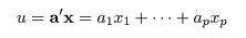
|
|
 |
 |
 |
|

|
|
|
 |

|
|
library(MASS) # MASS ライブラリィーの呼び出し
Cushings # Cushings データ
cush2 <- log(Cushings[1:16,1:2])
tp2 <- factor(Cushings$Type[1:16]) # カテゴリー変数化
cush2.lda <- lda(cush2, tp2) # 線形判別
cush2.qda <- qda(cush2, tp2) # 2次判別
Tetrahydrocortisone <- cush2[,1]
Pregnanetriol <- cush2[,2]
# ロジスティック回帰
cush2.glm <- glm(tp2 ~ Tetrahydrocortisone + Pregnanetriol, family=binomial)
#
# 散布図上の判別線表示
len <- 100
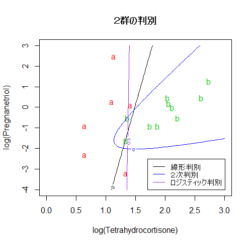
plot(cush2, type="n", xlim=c(0,3), ylim=c(-4,3),
xlab="log(Tetrahydrocortisone)", ylab="log(Pregnanetriol)")
text(cush2, as.character(tp2), col=as.numeric(tp2)+1)
title(main="2群の判別")
xp <- seq(0, 3, length = len)
yp <- seq(-4, 3, length = len)
# 100 × 100 のグリッドの定義
cushT <- expand.grid(Tetrahydrocortisone=xp, Pregnanetriol=yp)
Z <- predict(cush2.lda, cushT) # 線形判別でのグリッド上の事後確率
zp <- Z$posterior[,1] - Z$posterior[,2] # a の事後確率 − b の事後確率
contour(xp, yp, matrix(zp, len), add=T, levels=0) # 等事後確率線
#
Z <- predict(cush2.qda, cushT) # 2次判別でのグリッド上の事後確率
zp <- Z$posterior[,1] - Z$posterior[,2]
contour(xp, yp, matrix(zp, len), add=T, levels=0, col="blue")
#
Z <- predict(cush2.glm, cushT, type="response") # a の確率
contour(xp, yp, matrix(Z, len), add=T, levels=0.5, col="purple") # a が 0.5 になる線
legend("bottomright", legend=c("線形判別","2次判別","ロジスティック判別"),
lty=1, col=c("black","blue","purple"), cex=0.8)
 |
 |
 |
 |
cush <- log(Cushings[1:21,1:2])
tp <- factor(Cushings$Type[1:21])
len <- 100
xp <- seq(0, 4.5, length = len)
yp <- seq(-4, 3, length = len)
cushT <- expand.grid(Tetrahydrocortisone=xp, Pregnanetriol=yp)
#
# 判別線表示関数定義
predplot <- function(pred, main=""){
plot(cush, type="n", xlim=c(0,4.5), ylim=c(-4,3),
xlab="log(Tetrahydrocortisone)", ylab="log(Pregnanetriol)", main=main)
text(cush, as.character(tp), col=as.numeric(tp)+1)
zp <- pred[,3] - pmax(pred[,2], pred[,1])
contour(xp, yp, matrix(zp, len), add=T, levels=0)
zp <- pred[,1] - pmax(pred[,2], pred[,3])
contour(xp, yp, matrix(zp, len), add=T, levels=0)
}
#
#
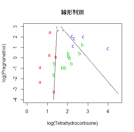
# 線形判別
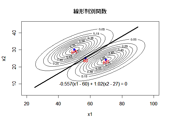
cush.lda <- lda(cush, tp) # 線形判別関数
Z <- predict(cush.lda, cushT)
main <- "線形判別"
predplot(Z$posterior, main=main)
#
# 2次判別
cush.qda <- qda(cush, tp)
Z <- predict(cush.qda, cushT)
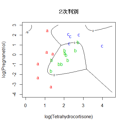
main <- "2次判別"
predplot(Z$posterior, main=main)
#
# 多項ロジスティック判別
Tetrahydrocortisone <- cush[,1]
Pregnanetriol <- cush[,2]
library(nnet)
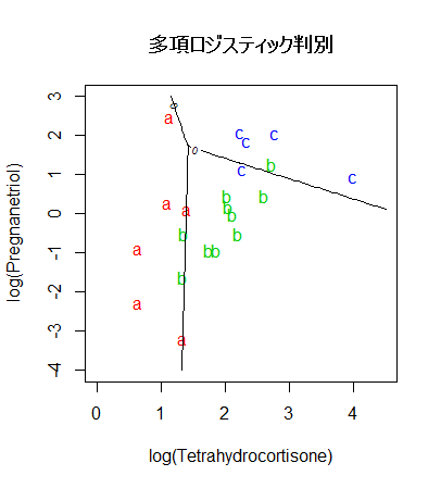
cush.multinom <- multinom(tp ~ Tetrahydrocortisone + Pregnanetriol, maxit=250)
zz <- predict(cush.multinom, cushT, type="probs")
main <- "多項ロジスティック判別"
predplot(zz, main=main)
#
# 決定木,分類木
library(rpart)
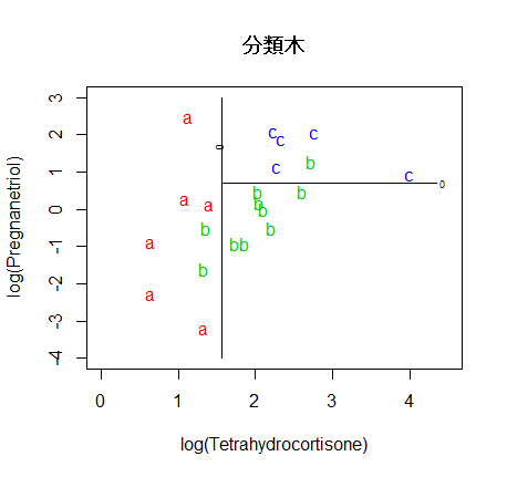
cush.tree <- rpart(tp ~ Tetrahydrocortisone + Pregnanetriol)
plot(cush.tree); text(cush.tree)
zz <- predict(cush.tree, cushT, type="prob")
main <- "分類木"
predplot(zz, main=main)
#
#
library(e1071)
# ナイーブベイズ(naive bayes)
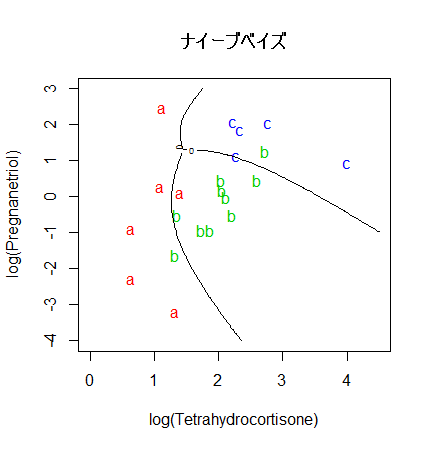
cush.bayes <- naiveBayes(cush, tp)
zz <- predict(cush.bayes, cushT, type="raw")
main <- "ナイーブベイズ"
predplot(zz, main=main)
#
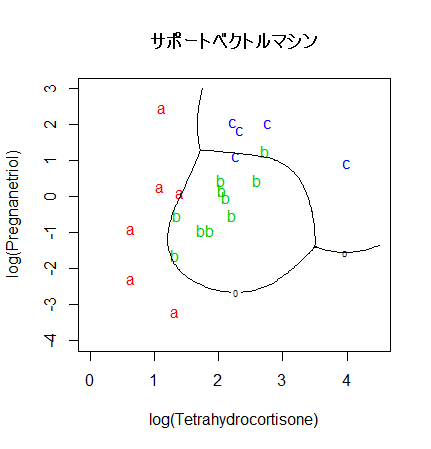
# サポートベクトルマシン(SVM)
cush.svm <- svm(tp ~ Tetrahydrocortisone + Pregnanetriol, probability = TRUE)
zz <- predict(cush.svm, cushT, decision.values = TRUE, probability = TRUE)
zz.dec <- attr(zz, "decision.values")
zz.prob <- attr(zz, "probabilities")
main <- "サポートベクトルマシン"
predplot(zz.prob, main=main)
#
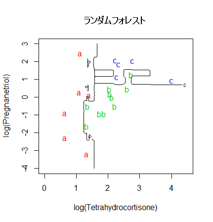
# ランダムフォレスト
library(randomForest)
set.seed(71)
cush.rf <- randomForest(cush, tp)
zz <- predict(cush.rf, cushT, type="prob")
main <- "ランダムフォレスト"
predplot(zz, main=main)
 |
 |
 |
 |
 |
 |
 |
|

|
library(MASS)
head(fgl)
nf <- which(fgl$type == "WinF")
nn <- which(fgl$type == "WinNF")
nv <- which(fgl$type == "Ven")
nc <- which(fgl$type == "Con")
nt <- which(fgl$type == "Tabl")
nh <- which(fgl$type == "Head")
type2 <- rep("", nrow(fgl))
type2[nf] <- "F"
type2[nn] <- "N"
type2[nv] <- "V"
type2[nc] <- "C"
type2[nt] <- "T"
type2[nh] <- "H"
typecol <- rep(0, nrow(fgl))
typecol[nf] <- 1
typecol[nn] <- 2
typecol[nv] <- 3
typecol[nc] <- 4
typecol[nt] <- 5
typecol[nh] <- 6
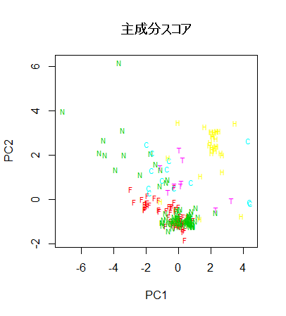
fgl.pca <- prcomp(scale(fgl[,-10]))
summary(fgl.pca)
plot(fgl.pca$x[,1:2], type="n")
text(fgl.pca$x[,1:2], type2, col=typecol+1, cex=0.7)
title(main="主成分スコア")
fgl.lda <- lda(type ~ ., data=fgl)
fgl.lda
fgl.pred <- predict(fgl.lda)
#
#
xp <- seq(-3.6,7.4, length=len)
yp <- seq(-8,3.8, length=len)
fglT <- expand.grid(LD1=xp, LD2=yp)
mld1 <- tapply(fgl.pred$x[,1], fgl$type, mean)
mld2 <- tapply(fgl.pred$x[,2], fgl$type, mean)
pred <- NULL
for(i in 1:nrow(fglT)){
d1 <- dnorm(fglT[i,1],mean=mld1, sd=1)
d2 <- dnorm(fglT[i,2],mean=mld2, sd=1)
pred <- rbind(pred, fgl.lda$prior*d1*d2/sum(fgl.lda$prior*d1*d2))
}
#
#
plot(fgl.pred$x[,1:2], type="n")
text(fgl.pred$x[,1:2], type2, col=typecol+1, cex=0.7)
title(main="正準判別スコアと判別境界")
#
# 判別境界表示
zp <- pred[,1] - pmax(pred[,2], pred[,3], pred[,4], pred[,5], pred[,6])
contour(xp, yp, matrix(zp, len), add=T, levels=0)
zp <- pred[,2] - pmax(pred[,1], pred[,3], pred[,4], pred[,5], pred[,6])
contour(xp, yp, matrix(zp, len), add=T, levels=0)
zp <- pred[,3] - pmax(pred[,1], pred[,2], pred[,4], pred[,5], pred[,6])
contour(xp, yp, matrix(zp, len), add=T, levels=0)
zp <- pred[,4] - pmax(pred[,1], pred[,2], pred[,3], pred[,5], pred[,6])
contour(xp, yp, matrix(zp, len), add=T, levels=0)
zp <- pred[,5] - pmax(pred[,1], pred[,2], pred[,3], pred[,4], pred[,6])
contour(xp, yp, matrix(zp, len), add=T, levels=0)
#
# データ,判別表
fgltab.lda <- table(fgl$type, fgl.pred$class)
fgltab.lda
1 - sum(diag(fgltab.lda))/sum(fgltab.lda)
#
#
# force predict to return class labels only
mypredict.lda <- function(object, newdata)
predict(object, newdata = newdata)$class
# 10-fold CV 10 回
library(ipred)
set.seed(41)
error.lda <- numeric(10)
for(i in 1:10) error.lda[i] <-
errorest(type ~ ., data = fgl,
model = lda, predict= mypredict.lda)$error
summary(error.lda)
#
#
# SVM
library(e1071)
fgl.svm <- svm(type ~ ., data = fgl)
# データ,判別表
fgltab.svm <- table(fgl$type, fitted(fgl.svm))
fgltab.svm
1 - sum(diag(fgltab.svm))/sum(fgltab.svm)
# 10-fold CV 10 回
set.seed(563)
error.SVM <- numeric(10)
for (i in 1:10) error.SVM[i] <-
errorest(type ~ ., data = fgl,
model = svm)$error
summary(error.SVM)
#
#
library(randomForest)
set.seed(17)
fgl.rf <- randomForest(type ~ ., data = fgl,
mtry = 2, importance = TRUE,
do.trace = 100)
print(fgl.rf)
fgltab.rf <- table(fgl$type, fgl.rf$predicted)
fgltab.rf
1 - sum(diag(fgltab.rf))/sum(fgltab.rf)
#
# 10-fold CV 10 回
library(ipred)
set.seed(131)
error.RF <- numeric(10)
for(i in 1:10) error.RF[i] <-
errorest(type ~ ., data = fgl,
model = randomForest, mtry = 2)$error
summary(error.RF)
#
 |
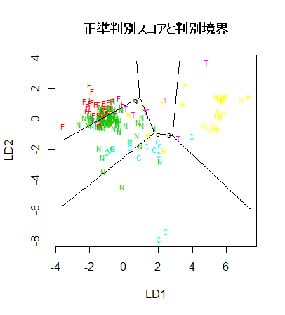 |
 正準判別
        WinF WinNF Veh Con Tabl Head
  WinF    52    15   3   0    0    0
  WinNF   17    54   0   3    2    0
  Veh     11     6   0   0    0    0
  Con      0     5   0   7    0    1
  Tabl     1     2   0   0    6    0
  Head     1     2   0   1    0   25
判別誤差:0.3271,予測誤差:0.3818

 SVM
        WinF WinNF Veh Con Tabl Head
  WinF    59    11   0   0    0    0
  WinNF   15    61   0   0    0    0
  Veh     10     7   0   0    0    0
  Con      0     0   0  13    0    0
  Tabl     0     1   0   0    8    0
  Head     1     0   0   0    0   28
判別誤差:0.2103,予測誤差:0.2935

 ランダムフォレスト
       WinF WinNF Veh Con Tabl Head
  WinF    63     6   1   0    0    0
  WinNF   11    61   1   1    2    0
  Veh      7     4   6   0    0    0
  Con      0     3   0   9    0    1
  Tabl     0     1   0   0    8    0
  Head     1     3   0   0    0   25
判別誤差:0.1916,予測誤差:0.2065