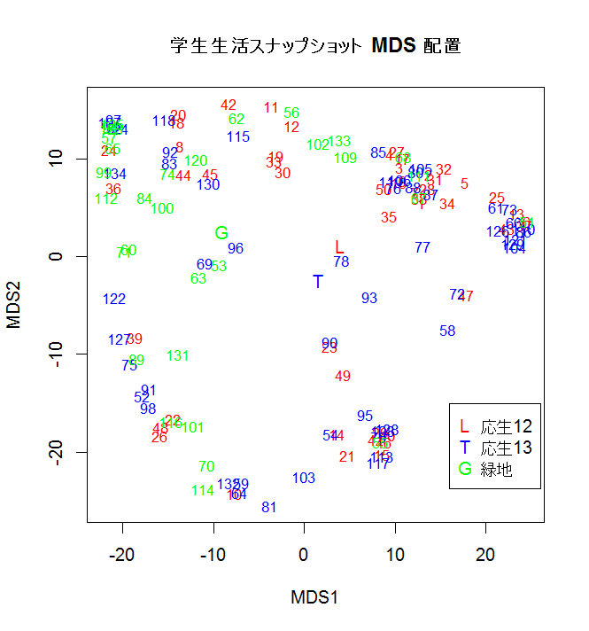
スナップショット配置と専修,年次
これも忘れずに
#### Def. of function ####
"%w/o%" <- function(x, y) x[!x %in% y] #-- x without y
#
mkmat <- function(wg){ # 0 - 1 行列を作成する関数の定義
n <- length(wg) # ベクトルの長さ(画像数)
maxg <- max(wg) # グループ最大値
ming <- min(wg) # グループ最小値(普通は1)
if(!ming){ # 最小値が 0 のときの処置
ming <- 1; maxg <- maxg+1; wg <- wg+1 # グループ数を 1 つ増やす
} #
gmat <- matrix(0, nrow=n, ncol=maxg) # n × maxg 行列(値は 0)
for(i in ming:maxg){ # グループごとの処理
ng <- (1:n)[wg == i] # グループ i に所属する行番号(画像番号)
gmat[ng, i] <- 1 # 上の行番号と i 列の値を 1 にする
} #
return(gmat) #
} #
#### End ###########
#w <- mkmat(tg[1, ]); w # 1 番目の学生のグルーピング行列
#apply(w, 2, sum) # 各グループのメンバー数
#
tg <- read.csv("lifegr13.csv", header=TRUE, row.names=1) # csv グルーピングデータ読み込み
n <- ncol(tg); n # 画像の数
m <- nrow(tg); m # 学生の数
data0 <- read.csv("data13.csv", header=TRUE, row.names=1)
b012 <- which(data0$year==12) # 12年度応用生物(緑地データ無し)
g0 <- which(data0$major == "G") # 13年度緑地
b013 <- (1:n)[-b012] %w/o% g0 # 13年度応用生物
S <- matrix(0, nrow=n, ncol=n) # 類似度行列の定義
for(i in 1:m){ #
w <- mkmat(tg[i, ]) # 学生ごとのグルーピング行列
S <- S + w %*% t(w) # 学生ごとの類似度行列を加える
} #
D <- max(S) - S # 非類似度行列への変換
tcmd <- cmdscale(D, k=4, eig=TRUE, add=TRUE) # 多次元尺度法(MDS)
tcmd$eig[1:4] # MDS の固有値
x <- tcmd$points # MDS の座標を x に格納
dimnames(x) <- list(as.character(1:n), paste("MDS", 1:4, sep="")) # x の列と行の名前を定義
plot(x[,1:2], type="n") # 1軸と2軸
text(x[b012,1:2], rownames(x)[b012], cex=0.8, col="red") # 昨年度学生生活写真番号
text(x[b013,1:2], rownames(x)[b013], cex=0.8, col="blue") # 今年度学生生活写真番号
text(x[g0,1:2], rownames(x)[g0], cex=0.8, col="green") # 緑地環境学
yl <- apply(x[b012,1:2],2,mean)
yt <- apply(x[b013,1:2],2,mean)
yg <- apply(x[g0,1:2],2,mean)
text(yl[1],yl[2], "L", col="red")
text(yt[1],yt[2], "T", col="blue")
text(yg[1],yg[2], "G", col="green")
legend(16,-15,legend=c("応生12","応生13","緑地"), pch=c("L","T","G"), col=c("red","blue","green"))
title(main="学生生活スナップショット MDS 配置")
#
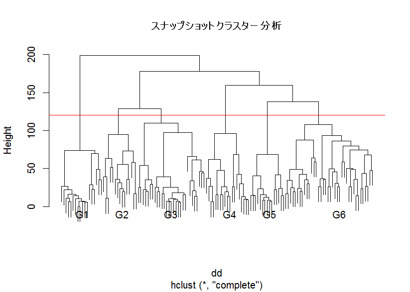
dd <- dist(D)
dd.clus <- hclust(dd)
plot(dd.clus, cex=0.4, labels = FALSE, main="スナップショットクラスター分析")
abline(h=120, col="red")
text(10,-10,"G1")
text(27,-10,"G2")
text(48,-10,"G3")
text(73,-10,"G4")
text(90,-10,"G5")
text(120,-10,"G6")
wclass <- cutree(dd.clus, h=120)
table(wclass)
ncla <- length(table(wclass))
ncla # 6 クラスター
#
group0 <- read.csv("group.csv", header=TRUE, row.names=1)
group <- group0[,1]
g1 <- which(group==1)
g2 <- which(group==2)
g3 <- which(group==3)
g4 <- which(group==4)
g5 <- which(group==5)
g6 <- which(group==6)
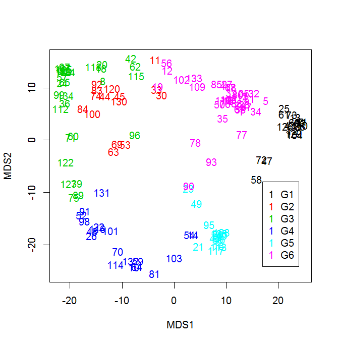
plot(x[,1:2], type="n") # 1軸と2軸
text(x[g1,1:2], rownames(x)[g1], col=1)
text(x[g2,1:2], rownames(x)[g2], col=2)
text(x[g3,1:2], rownames(x)[g3], col=3)
text(x[g4,1:2], rownames(x)[g4], col=4)
text(x[g5,1:2], rownames(x)[g5], col=5)
text(x[g6,1:2], rownames(x)[g6], col=6)
gname <- c(paste("G",1:6,sep=""))
legend(18,-9,legend=gname, pch="1",col=1:6)
#
major <- rep("",n)
major[b012] <- "L"
major[b013] <- "T"
major[g0] <- "G"
tab <- table(major, group); tab
chisq.test(tab)
tab[-1,]
chisq.test(tab[-1,])
写真つき類似度マップをみるとわかりやすい.
text0 <- read.csv("text.csv", row.names=1, header=T)
word0 <- read.csv("word.csv", row.names=1, header=T)
cut <- which(word0$cut==1)
text <- text0[-cut,]
word <- word0[-cut,]
dim(text)
rownames(text)
# 同義語をまとめる
m11 <- which(rownames(text)=="控え室"); m11
m12 <- which(rownames(text)=="控室"); m12
drop <- m11
text2 <- text
text2[m12,] <- text[m11,]+text[m12,]
text2 <- text2[-drop,]
word2 <- word[-drop,]
# 他の同義語もまとめてみよう。
#
# 単語0の列を除く
colnames(text2) <- rownames(data0)
noword <- which(apply(text2,2,sum)==0)
txtcut <- c(which(data0$remark==1), noword)
text3 <- text2[,-txtcut]
group3 <- group[-txtcut]
major3 <- major[-txtcut]
g1 <- which(group3==1)
g2 <- which(group3==2)
g3 <- which(group3==3)
g4 <- which(group3==4)
g5 <- which(group3==5)
g6 <- which(group3==6)
b12 <- which(major3=="L")
b13 <- which(major3=="T")
green <- which(major3=="G")
# 0-1化
radj.vec <- as.vector(as.matrix(text3))
vexsist <- which(radj.vec >0)
radj.vec[vexsist] <- 1
text01 <- matrix(radj.vec, nrow=nrow(text3))
rownames(text01) <- rownames(text3)
colnames(text01) <- colnames(text3)
cbind(apply(text3, 1, sum), apply(text01, 1, sum))
#
wg1 <- apply(text01[,g1],1,sum)
wg2 <- apply(text01[,g2],1,sum)
wg3 <- apply(text01[,g3],1,sum)
wg4 <- apply(text01[,g4],1,sum)
wg5 <- apply(text01[,g5],1,sum)
wg6 <- apply(text01[,g6],1,sum)
wb12 <- apply(text01[,b12],1,sum)
wb13 <- apply(text01[,b13],1,sum)
wgreen <- apply(text01[,green],1,sum)
#
text.all <- cbind(wg1,wg2,wg3,wg4,wg5,wg6,wb12,wb13,wgreen,text01)
mm <- ncol(text.all); mm
library(MASS)
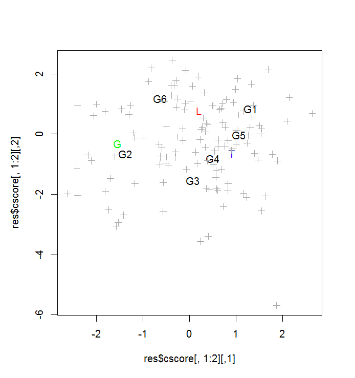
res <- corresp(log(text.all+1), nf=4)
res$cor
biplot(res)
plot(res$cscore[,1:2], type="n")
text(res$cscore[1:6,1:2], gname)
text(res$cscore[7:9,1:2], c("L","T","G"), col=c("red","blue","green"))
points(res$cscore[10:mm,1:2],pch=3, col="darkgrey")
unique <- which(word2$unique==1)
feel <- which(word2$feel==1)
rownames(text01)[unique]
rownames(text01)[feel]
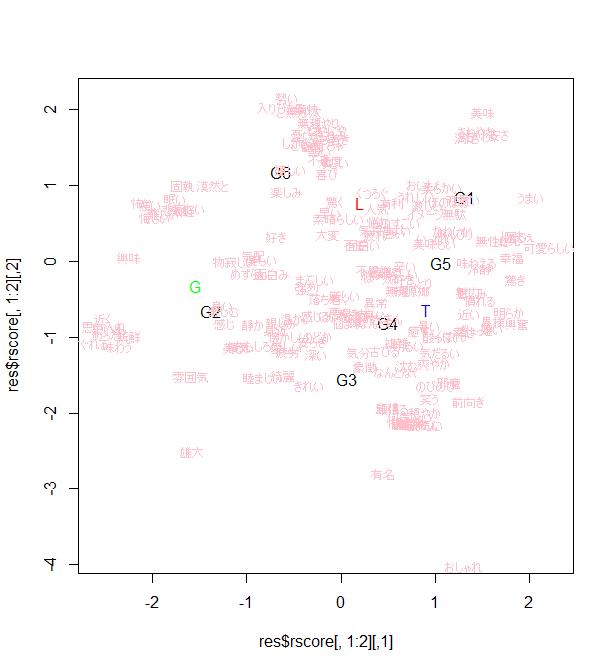
plot(res$rscore[,1:2], type="n")
text(res$cscore[1:6,1:2], gname)
text(res$cscore[7:9,1:2], c("L","T","G"), col=c("red","blue","green"))
text(jitter(res$rscore[feel,1:2],amount=0.2), rownames(res$rscore)[feel], cex=0.7, col="pink")
# G1 でよく使われた単語
sort(wg1, decreasing=T)[1:50]
# 緑地でよく使われた単語
sort(wgreen, decreasing=T)[1:50]
課題:
1.各グループのタイトルと代表写真,よく使われた特徴的と思われる単語。
2.応生と緑地での違い。
3.よく使われた特徴的と思われる単語を用い応生の生活を紹介する文章と対応する写真を2,3点のせる。