東京大学大学院農学生命科学研究科　大森宏

http://lbm.ab.a.u-tokyo.ac.jp/~omori/experiment12/zissyu.html

実習基本情報

2016耕種概要と品種
収量構成要素の説明
第１回配布プリント
2015耕種概要と品種（参考）

データ

2016年度

エクセルデータダウンロード(AllData2016.xlsx)
Ｒ用データダウンロード(Rice2016.csv)

2015年度（参考）

エクセルデータダウンロード(AllData2015.xlsx)
Ｒ用データダウンロード(Rice2015.csv)

収量の分散分析

とおける．ただし，μ は総平均，α_i は品種効果，β_j は栽植密度，(αβ)_ij は 品種と栽植密度の交互作用，ρ_k はブロック効果， ｅ_ijk は誤差である． 誤差項は，ｅ_ijk 〜 N（0，σ²）を満たす互いに独立な変量（確率変数）であるとする．

# データ読み込み
rice0 <- read.csv("Rice2016.csv") 
names(rice0)	# 変数名
#品種，栽植密度，ブロック, でソート
rice <- rice0[order(rice0$Variety, rice0$Pl_Density_m2, rice0$Replication),]
dim(rice)	# 30 39
# 各処理を因子にする
variety <- factor(rice$Variety)
levels(variety)
density <- factor(rice$Pl_Density_m2)
levels(density)
rep <- factor(rice$Replication)
# 収量の分散分析
y <- rice$GrainYield_gm2
summary(aov(y ~ variety + density + variety:density + rep))
# 収量のグラフ
vy <- tapply(y, variety, mean); vy		# 品種ごとの平均
o <- order(vy, decreasing=T)
vy[o]			# 大きい順に表示
tapply(y, density, mean)		# 栽植密度ごとの平均
# 栽植密度と品種組み合わせごとの平均
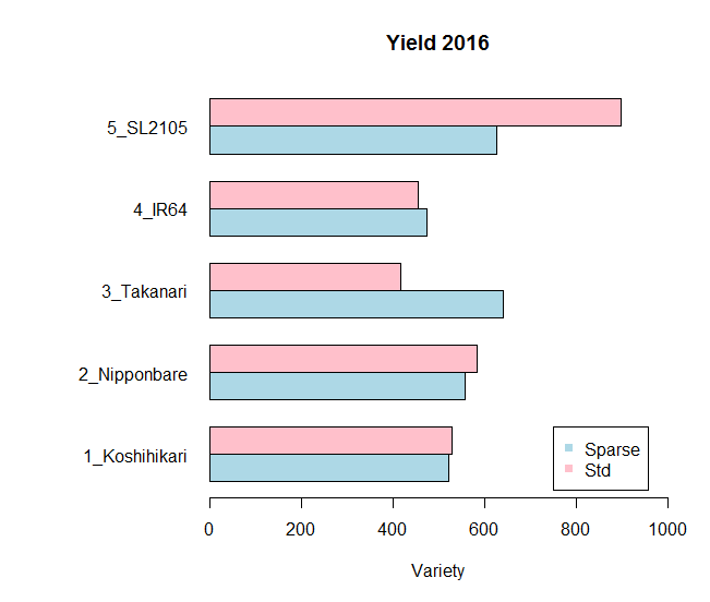
x <- tapply(y, density:variety, mean); x
xx <- rbind(x[1:5], x[6:10])
rownames(xx) <- c("Sparse","Std")
colnames(xx) <- levels(variety)
op <- par(mar=c(5,10,4,2))		# 左余白を広くする(10)
barplot(xx, beside=TRUE, horiz=TRUE, xlab="Variety", ylab="", las=TRUE,
	xlim=c(0,1000),col=c("lightblue","pink"))
legend(750, 3, legend=c("Sparse","Std"), pch=15, col=c("lightblue","pink") )
title(main="Yield 2016")
par(op)

                Df Sum Sq Mean Sq F value  Pr(>F)   
variety          4 308861   77215   5.535 0.00437 **
density          1   1169    1169   0.084 0.77548   
rep              2  47826   23913   1.714 0.20824   
variety:density  4 185198   46299   3.319 0.03339 * 
Residuals       18 251103   13950                   

# 形質間相関
names(rice)
# 7月生育調査 5,6,7,8
# 10月収穫調査 13-39
names(rice[,c(5:8,c(32:33,37:39))])
cor(rice[,c(5:8,c(32:33,37:39))])
pairs(rice[,c(6:8,c(32:33,37:39))])

回帰分析

y <- rice$GrainYield_gm2
x1 <- rice$StemNumber_Jul_m2
x2 <- rice$PlantHeight_cm_Jul
x3 <- rice$SPAD_Jul
res3 <- lm(y ~ x1+x2+x3)
summary(res3)
# x3 はいらないかも
res2 <- lm(y ~ x1+x2)
summary(res2)
anova(res2, res3)
# x2 もいらないかも
res1 <- lm(y ~ x1)
summary(res1)
anova(res1, res2)
anova(res1, res3)

> summary(res3)

Call:
lm(formula = y ~ x1 + x2 + x3)

Residuals:
    Min      1Q  Median      3Q     Max 
-382.04  -84.12    6.65   96.58  235.23 

Coefficients:
             Estimate Std. Error t value Pr(>|t|)  
(Intercept) -509.7305   485.1467  -1.051   0.3031  
x1             0.6418     0.2456   2.613   0.0147 *
x2             7.2041     4.0042   1.799   0.0836 .
x3            11.3062    10.3838   1.089   0.2862  
---
Signif. codes:  0 ‘***’ 0.001 ‘**’ 0.01 ‘*’ 0.05 ‘.’ 0.1 ‘ ’ 1

Residual standard error: 148.3 on 26 degrees of freedom
Multiple R-squared:   0.28,     Adjusted R-squared:  0.197 
F-statistic: 3.371 on 3 and 26 DF,  p-value: 0.03356

レポートについて

sasaki@isas.a.u-tokyo.ac.jp